3.8. Script 8: Primary Education Fate¶

Primary Education is modeled in a multi-step way. This code calculates the study fate (never entered, dropout, graduated) by sex and district and constitutes the base model of primary education. It can be complemented by more detailed fate models introducing relative factors accounting for additional individual level differences, as well as models for tracking students through the education system.

The code below calculates school entry and graduation parameters for a cohort model by sex and district of birth. The two model parameters are stored in a Modgen .dat file

School entry by district of birth, sex and year of birth
School retention by district of birth, sex and year of birth

3.8.1. Code¶

3.8.1.1. School Entry¶

####################################################################################################
# 
#  DYNAMIS-POP Parameter Generation File 8 Chunk A - Primary Education School Entry
#  This file is generic and works for all country contexts. 
#  Input file: globals_for_analysis.RData (To generate such a file run the setup script)
#  Last Update: Martin Spielauer 2018-06-29
#
####################################################################################################

####################################################################################################
# Clear work space, load required packages and the input object file
####################################################################################################

rm(list=ls())

library(haven)
library(dplyr)
library(data.table)
library(sp) 
library(maptools)
library(survival)
library(fmsb)
library(eha)

load(file="globals_for_analysis.RData")
parafile        <- file(g_para_primaryeduc, "w") # Output Parameter File
dat             <- g_residents_dat               # Main data object for education analysis

# Constants

n_maxdist       <- max(dat$M_DOB)
n_maxdistP1     <- n_maxdist + 1
n_maxreg        <- max(dat$M_ROB)
n_maxregP1      <- n_maxreg + 1

# Add some variables

dat$m_age       <- as.integer(dat$M_AGE)
dat$m_any_educ  <- as.logical(dat$M_EDUC > 0)
dat$m_finish    <- as.logical(dat$M_EDUC > 1)
dat$M_WEIGHT    <- dat$M_WEIGHT / g_reweight

####################################################################################################
# Model school Entry by region
####################################################################################################

# remove those out of age range 12-32

dat <- dat[!(dat$m_age < 12),]
dat <- dat[!(dat$m_age > 32),]

# logistic regression school entry male

MaleEntry        <- glm(m_any_educ ~ m_age+factor(M_ROB), family = quasibinomial, weights = M_WEIGHT, data = dat[dat$M_MALE==1,])
MaleEntryPredict <- predict(MaleEntry,data.frame(m_age=rep(11:-51,each=n_maxregP1),M_ROB=rep(0:n_maxreg,63)))
MaleEntryPredict <- exp(MaleEntryPredict) / (1+exp(MaleEntryPredict))

# logistic regression school entry female

FemEntry        <- glm(m_any_educ ~ m_age+factor(M_ROB), family = quasibinomial, weights = M_WEIGHT, data = dat[dat$M_MALE==0,])
FemEntryPredict <- predict(FemEntry,data.frame(m_age=rep(11:-51,each=n_maxregP1),M_ROB=rep(0:n_maxreg,63)))
FemEntryPredict <- exp(FemEntryPredict) / (1+exp(FemEntryPredict))

####################################################################################################
# Write Parameters school Entry by region - NOT USED
####################################################################################################

cat("parameters  {\n", file=parafile)
#cat("parameters  {\n\n//EN School entry\ndouble  StartPrimary[SEX][YOB_START_PRIMARY][PROVINCE_INT] = {\n", file=parafile)
#cat(format(round(FemEntryPredict,7),scientific=FALSE), file=parafile, sep=", ", append=TRUE)
#cat(",\n", file=parafile, append=TRUE)
#cat(format(round(MaleEntryPredict,7),scientific=FALSE), file=parafile, sep=", ", append=TRUE)
#cat("\n}; \n\n", file=parafile, append=TRUE) 


####################################################################################################
# Model School Entry By Districts
####################################################################################################

# logistic regression school entry male

MaleEntry        <- glm(m_any_educ ~ m_age+factor(M_DOB), family = quasibinomial, weights = M_WEIGHT, data = dat[dat$M_MALE==1,])
MaleEntryPredict <- predict(MaleEntry,data.frame(m_age=rep(11:-51,each=n_maxdistP1),M_DOB=rep(0:n_maxdist,63)))
MaleEntryPredict <- exp(MaleEntryPredict) / (1+exp(MaleEntryPredict))

# logistic regression school entry female

FemEntry        <- glm(m_any_educ ~ m_age+factor(M_DOB), family = quasibinomial, weights = M_WEIGHT, data = dat[dat$M_MALE==0,])
FemEntryPredict <- predict(FemEntry,data.frame(m_age=rep(11:-51,each=n_maxdistP1),M_DOB=rep(0:n_maxdist,63)))
FemEntryPredict <- exp(FemEntryPredict) / (1+exp(FemEntryPredict))

####################################################################################################
# Write Parameters School Entry By Districts
####################################################################################################

cat("\n\n//EN School entry by district\ndouble  StartPrimaryDistrict[SEX][YOB_START_PRIMARY][DISTRICT_INT] = {\n", file=parafile, append=TRUE)
cat(format(round(FemEntryPredict,7),scientific=FALSE), file=parafile, sep=", ", append=TRUE)
cat(",\n", file=parafile, append=TRUE)
cat(format(round(MaleEntryPredict,7),scientific=FALSE), file=parafile, sep=", ", append=TRUE)
cat("\n}; \n\n", file=parafile, append=TRUE) 

####################################################################################################
# Map Illustration current preobabilities (children currently age 12)
####################################################################################################

male_vector   <- head(MaleEntryPredict,length(g_shape_display_order))
female_vector <- head(FemEntryPredict,length(g_shape_display_order))

country_shape <- rgdal::readOGR(g_shapes)

## Districts as coded in Census in the order of districts in the country shape object 
country_shape$censusdist <- g_shape_display_order

## Function taking a SpatialPolygonsDataFrame and adding a vector of values to be displayed on map
## The values come in the order of provinces as coded in the census and are re-ordered to fit the 
## Country shape object

AddVectorForDisplay <- function(country_shape,VectorForDisplay) 
{
  testb          <- data.frame(cbind(new_order=country_shape$censusdist,orig_order=c(0:max(g_shape_display_order))))
  testb          <- testb[order(testb$new_order),]
  testb$newcol   <- VectorForDisplay
  testb          <- testb[order(testb$orig_order),]
  country_shape$graphval <- testb$newcol
  return(country_shape)
}

## The code to plot data 
spplot(AddVectorForDisplay(country_shape,male_vector),c("graphval"), at = c(0.0, 0.10, 0.2, 0.3, 0.4,0.5, 0.6,0.7, 0.8, 0.9, 1),main = "Male Primary Entry" )
spplot(AddVectorForDisplay(country_shape,female_vector),c("graphval"), at = c(0.0, 0.10, 0.2, 0.3, 0.4,0.5, 0.6,0.7, 0.8, 0.9, 1),main = "Female Primary Entry" )

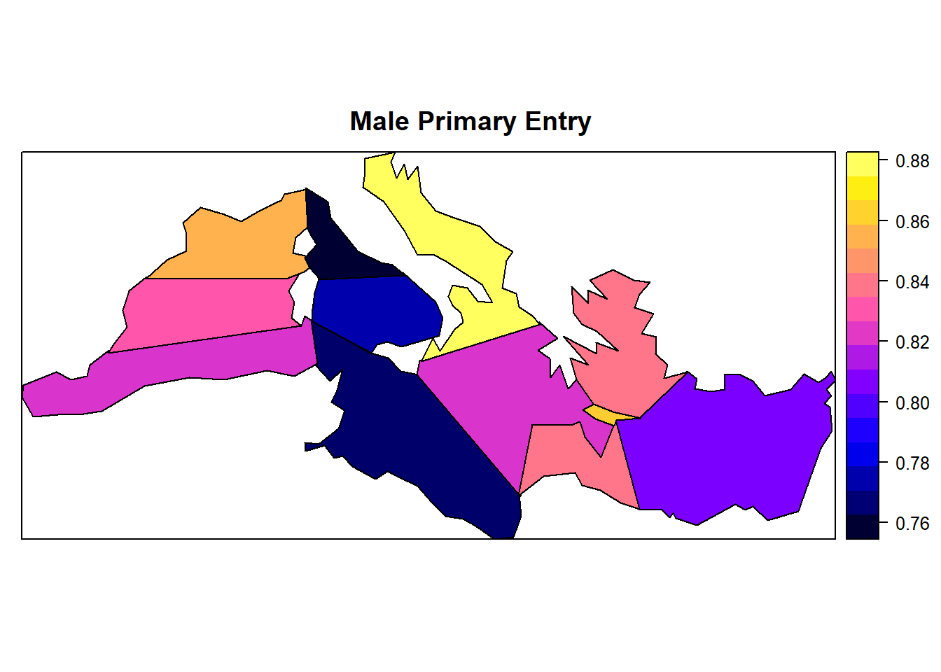../../_images/08_01.png Figure: Male Primary Entry 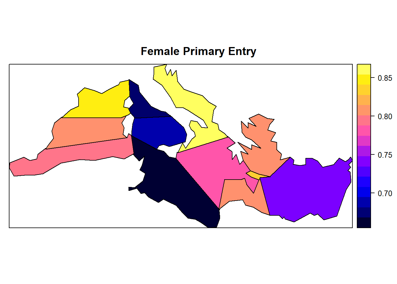../../_images/08_02.png Figure: Female Primary Entry

3.8.1.2. School Retention¶

####################################################################################################
# 
#  DYNAMIS-POP Parameter Generation File 8 Chunk B - Primary Education School Retention
#
####################################################################################################

####################################################################################################
# Model school retention by region
####################################################################################################

# remove those out of age range < 16 and those who never entered

dat <- dat[!(dat$m_age < 16),]
dat <- dat[(dat$m_any_educ == TRUE),]

# logistic regression school entry male

MaleFinish        <- glm(m_finish ~ m_age+factor(M_ROB), family = quasibinomial, weights = M_WEIGHT, data = dat[dat$M_MALE==1,])
MaleFinishPredict <- predict(MaleFinish,data.frame(m_age=rep(15:-51,each=n_maxregP1),M_ROB=rep(0:n_maxreg,67)))
MaleFinishPredict <- exp(MaleFinishPredict) / (1+exp(MaleFinishPredict))

# logistic regression school entry female

FemFinish        <- glm(m_finish ~ m_age+factor(M_ROB), family = quasibinomial, weights = M_WEIGHT, data = dat[dat$M_MALE==0,])
FemFinishPredict <- predict(FemFinish,data.frame(m_age = rep(15:-51,each=n_maxregP1),M_ROB=rep(0:n_maxreg,67)))
FemFinishPredict <- exp(FemFinishPredict) / (1+exp(FemFinishPredict))

####################################################################################################
# Write parameters for school retention by region - NOT USED
####################################################################################################

#cat("\n\n//EN School retention\ndouble  GradPrimary[SEX][YOB_GRAD_PRIMARY][PROVINCE_INT] = {\n", file=parafile, append=TRUE)
#cat(format(round(FemFinishPredict,7),scientific=FALSE), file=parafile, sep=", ", append=TRUE)
#cat(",\n", file=parafile, append=TRUE)
#cat(format(round(MaleFinishPredict,7),scientific=FALSE), file=parafile, sep=", ", append=TRUE)
#cat("\n}; \n\n", file=parafile, append=TRUE) 

####################################################################################################
# Model School Retention By Districts
####################################################################################################

MaleFinish        <- glm(m_finish ~ m_age+factor(M_DOB), family = quasibinomial, weights = M_WEIGHT, data = dat[dat$M_MALE==1,])
MaleFinishPredict <- predict(MaleFinish,data.frame(m_age=rep(15:-51,each=n_maxdistP1),M_DOB=rep(0:n_maxdist,67)))
MaleFinishPredict <- exp(MaleFinishPredict) / (1+exp(MaleFinishPredict))

# logistic regression school entry female

FemFinish        <- glm(m_finish ~ m_age+factor(M_DOB), family = quasibinomial, weights = M_WEIGHT, data = dat[dat$M_MALE==0,])
FemFinishPredict <- predict(FemFinish,data.frame(m_age = rep(15:-51,each=n_maxdistP1),M_DOB=rep(0:n_maxdist,67)))
FemFinishPredict <- exp(FemFinishPredict) / (1+exp(FemFinishPredict))

####################################################################################################
# Write parameters for School Retention By Districts
####################################################################################################

cat("\n\n//EN School retention\ndouble  GradPrimaryDistrict[SEX][YOB_GRAD_PRIMARY][DISTRICT_INT] = {\n", file=parafile, append=TRUE)
cat(format(round(FemFinishPredict,7),scientific=FALSE), file=parafile, sep=", ", append=TRUE)
cat(",\n", file=parafile, append=TRUE)
cat(format(round(MaleFinishPredict,7),scientific=FALSE), file=parafile, sep=", ", append=TRUE)
cat("\n  }; ", file=parafile, append=TRUE) 
cat("\n};\n", file=parafile, append=TRUE) 
close(parafile)

####################################################################################################
# Map Illustration current retention (children currently age 12)
####################################################################################################

male_vector   <- head(MaleFinishPredict,length(g_shape_display_order))
female_vector <- head(FemFinishPredict,length(g_shape_display_order))

country_shape <- rgdal::readOGR(g_shapes)

## Census districts as coded in Census in the order of districts in the Nepal shape object (ID_3)
country_shape$censusdist <- g_shape_display_order

## The code to plot data 
spplot(AddVectorForDisplay(country_shape,male_vector),c("graphval"), main = "Male Primary Retention" )
spplot(AddVectorForDisplay(country_shape,female_vector),c("graphval"), main = "Female Primary Retention")

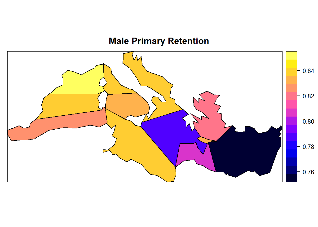../../_images/08_03.png Figure: Male Primary Retention 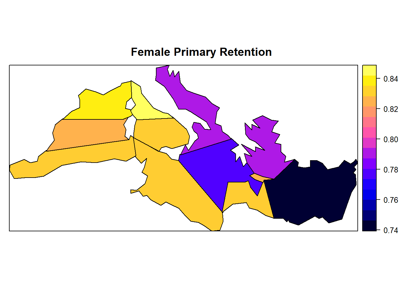../../_images/08_04.png Figure: Female Primary Retention