2.3. Modules, Parameters and Table Output¶

2.3.1. Starting Population¶

2.3.1.1. Model Overview¶

DYNAMIS-POP creates a simulated population based on a starting population micro-data file. The simulation size is chosen by the user. It can be smaller or larger than the micro-data file, DYNAMIS-POP automatically generates the simulated population from the file. If and how often a record is sampled depends on its weight, the size of the file, and the size of the simulation. While the records of the micro-data can be weighted, all simulated persons have the same weight. Parameters contain the necessary information for the creation of the simulated population.

2.3.1.2. Parameters¶

Simulated sample size of starting population: This parameter gives users the choice to set the size of the simulation. The smaller the size, the faster the simulation but also its the higher its randomness. The appropriate simulation size depends on the size of the studied population group and the likeliness of studied events. For example, projecting the total population number will require a smaller sample than projecting the number of school dropouts on a district level. In practice, a population size of 100,000 is sufficient for most preliminary analysis; Results on immunization published in Spielauer & Dupriez (2020) are based on 24 replicates with a initial population of 250,000 each. The table output of the model provides distributional information - e.g. the coefficient of variation - measuring the Monte-Carlo variability of each table cell which helps determining an appropriate simulation size. (A typical criterion is keeping the coefficient of variation below one percent for key outputs.)
File name of starting population
File size of starting population: The number of records to be read. This is usually the size of the file, but users can also choose a smaller number which might be useful (more computational efficient) if the file is very large and only a small simulation run based on a subset of the data is intended. (In this case, the order of records should be random)
Real population size: The real population size. All output of DYNAMIS-POP is automatically scaled to the real population size.

2.3.1.3. General Population Tables¶

Total population by sex and district
Total population by sex and region
Age Pyramids by District: Age pyramids using 5-year age groups (by sex and region).

2.3.2. Fertility¶

2.3.2.1. Model Overview¶

DYNAMIS-POP models fertility in two alternative ways and allows various ways of alignment. The first - the base model - is a replication of a typical population projection model driven by age specific fertility rates. In this approach fertility only depends on age and calendar year. The limitation of this “macro” approach is, that even having perfect foresight, besides for age, the distribution of children to women is not realistic as it does not account for factors like parity (the number of births a woman already had), spacing (time since last birth), partnership status, regional differences, or differences in timing and the distribution of family size by education. All these factors are accounted for in the second modeling approach implemented in DYNAMIS-POP. This “micro” approach - the refined model - uses a system of separate equations by parity. First births are based on rates by age, education, region, and partnership status. Higher order births use statistical models accounting for age, the time since last birth, and education. The second model also allows to model general time trends by parity. As changes in fertility are modeled explicitly, simulated changes can be decomposed to underlying factors like the changing education composition of mothers, changes in the distribution of the age of first marriage, and time trends. In the simulation children are linked to their mothers. Accounting for mothers’ characteristics in the fertility equations allows to include these characteristics when modeling processes like child mortality, immunization, and educational attainments.

As official population projections are typically performed using the first approach and the ability to reproduce these demographic scenarios might be desirable for many policy applications, DYNAMIS-POP provides alignment mechanisms which combine the two modelling approaches. In this case, total outcomes - either the total number of births, or the number of births by age - are consistent with the first model, while the second model is used to account for the fertility differences between women. When choosing alignment, the relative fertility differences between women of different characteristics remain unchanged, but rates are proportionally adjusted to meet the desired aggregate outcome. This is done automatically in the simulation.

2.3.2.2. User Options¶

Fertility model selection: there are four choices of how fertility is simulated
- Macro model (age only) - selecting this option, the macro - or base - model implementing age specific fertility like in cohort-component methods is applied. In this mode DYNAMIS-POP produces a typical macro model and therefore can reproduce published/official fertility projections. As this approach does not produce a realistic distribution of family sizes and does not account for individual level fertility differentials except or age, it should not be used when studying processes for which mothers’ characteristics are of importance, like child mortality, prenatal care, the intergenerational transmission of education, or immunization.
- Micro model un-aligned - selecting this option, the refined fertility model is used as is, thus without alignment to given outcomes. This option should be used if you trust the model (and underlying micro-data from which parameters are estimated) and there is no need to exactly reproduce given projections, but rather you use DYNAMIS-POP for exploring the down-stream effects of changes in other processes (e.g. educational expansion) on fertility.
- Micro model with aligned number of births - selecting this option, the refined fertility model is used, but the resulting number of births is aligned to the macro model. This option should be used if the alignment is a scenario requirement while a realistic distribution of births to women based on the detailed model is maintained as far as possible. While this approach does not allow the study of downstream effects of other processes on the number of births (which is given), it does allow studying changes in age patterns.
- Micro model with aligned number of births by age - With this alignment option, not only the number, but also the age distribution of mothers is aligned to the macro model. This option should be chosen if one aims at exactly reproducing the macro approach, while simultaneously distributing births realistically to women of a given age.

2.3.2.3. General Parameters¶

Sex Ratio (males per 100 females) by calendar year.

2.3.2.4. Parameters of the Base Model¶

Like in most population projection models, fertility in the base version of DYNAMIS-POP is driven by projected Age-Specific Fertility Rates (ASFRs) - the average number of children born to a woman by year of age. ASFRs contain two pieces of information: the age shape of birth risks and - summed up - the Total Fertility Rate (TFR) - the number of children that would be born to a woman over her lifetime if she was to experience the age-specific fertility rates for a given year through her lifetime (and assuming her survival over the reproductive age range). DYNAMIS-POP keeps this information in two separate parameters which provides an easy way of creating alternative scenarios on future TFRs without having to manipulate large distributional tables. In the simulation, each year ASFRs are calculated combining the information of the age distribution of fertility with the TFR.

Age distribution of fertility (for ages 10-49 by calendar year). This parameter contains the information of the relative age differences in fertility by age. Parameters can be expressed as the expected number of births by women of a given age (ASFRs). As only the relative differences in rates is used in the model, it is not required that parameters add up to TFR; a common way to express age specific patterns is to proportionally adjust the age specific rates in a way that they add up to one.
Total Fertility Rate (TFR) by calendar year. The number of children that would be born to a woman over her lifetime based on the ASFRs of a given calendar year.

2.3.2.5. Parameters of the Refined Model¶

First birth rates (by age, population group, geographical unit, and partnership status) Population groups and geographical units are country context specific. Default classifications are population groups by primary education attainment and a geographical classification by region.
Higher order births (by time since last birth, age group and education; separately by parity). Parameters are estimated using proportional (piecewise constant hazard regression) models. Birth risks are calculated by multiplying the baseline risk (by duration since last birth) with applicable relative risks (e.g. of being age 30-35 and having graduated from primary school).
Birth Trends (by parity and calendar year). This are trend parameters interpreted as additional relative risks. In the default setting all parameters are 1 assuming no trends.

2.3.2.6. Tables¶

Fertility rates and births by age. Displays age-specific fertility rates (ASFRs) and the absolute number of births by age for each simulated calendar year.
Births by mothers education. The absolute number of births by mothers education and district by year.
Average age at birth by education. The average age at first birth and at all births by education and year.
Births by district and age of mother. Number of births by age group for singling out very early and early teenage births. Numbers by district and year.
Proportion of births by mothers who never entered school by district and year.

2.3.2.7. Scenario Examples¶

Composition effects versus trends: The base fertility model projects a decrease of the TFR as specified in the parameter. The refined model allows to run a projection without trends, changes in fertility resulting only from the changing composition of women (most importantly by education). Such a scenario can be created by running the refined model without trends and without alignment.
Trend towards a 2 child family: Such a scenario can be created by including a negative trend for third and higher order births.
Downstream effects: A typical use of DYNAMSI-POP is the assessment of downstream effects, e.g of an educational expansion, on fertility. While these scenarios do not make changes in fertility parameters, be sure the refined model version without alignment is selected.

2.3.3. Mortality¶

2.3.3.1. Model Overview¶

Concerning mortality, the focus of DYNAMIS-POP (currently) lies on child mortality. While overall mortality is implemented in a way resembling typical population projection models being based on life tables, child mortality is modeled in more detail, accounting for mothers’ characteristics like her education and age at birth. The detailed model of child mortality is optional and - for an initial year - can be aligned to the base model. Users can also choose to apply separate trends for child mortality, or apply the overall trends calculated from the general changes in life expectancy.

2.3.3.2. User Options¶

Child mortality model selection: There are four alternative ways mortality is modeled:
- Disable child mortality model: The base model is used for all ages. This option should be chosen if child mortality is not subject of the simulation analysis and it is intended to exactly reproduce given population projections.
- Child mortality model without alignment: The refined child mortality model is used for children age 0-4. In this mode, no adjustments are made to the refined model. Changes in child mortality result from the changing educational and age composition of mothers and - if used - trends specified by the user.
- Aligned, trends as for other ages: In this mode, child mortality is aligned in the first year of simulation resulting in the same age-specific mortality rates as in the base model. From there on, changes result from the changing composition of mothers and from an overall trend similar to the trend applied in the base model. This general trend results from the improvement in life expectancy, which is a model parameter. This mode allows the study of downstream effects of improvements in mother’s education and the avoidance of early teenage pregnancies assuming that these improvements realize in addition to general trends affecting all ages.
- Aligned, trends from child mortality model: In this mode, child mortality is aligned in the first year of simulation resulting in the same age-specific mortality rates as in the base model. In the following years, trends specific to child mortality by year of age can be applied. Changes in child mortality result from the changing educational and age composition of mothers and - if used - trends specified by the user. This option allows making own assumptions on child mortality trends or - when not applying trends - to study composition effects in isolation.

2.3.3.3. Parameters of the Base Model¶

Like in most population projection models, mortality in the base version of DYNAMIS-POP is driven by a life table containing the age specific hazard rates of death. Life tables contain two pieces of information: the age profile of mortality risks and the remaining life expectancy at any year of age - most importantly the life expectancy at birth. DYNAMS-POP keeps this information in two separate parameters which provides an easy way of creating alternative scenarios on improvements in life expectancy without having to manipulate the hazard rates of the life table. This allows to use (and interprets the parameter as) standard life tables. During the simulation the standard life table is automatically scaled in order to meet life expectancy targets.

Life Table (age profile of hazards): The standard life table by sex.
Life Expectancy by sex. The period life expectancy of each calendar year by sex.

2.3.3.4. Parameters of the Refined Child Mortality Model¶

Child mortality baseline risks: the age specific baseline mortality for children (of the reference group, i.e. mother’s age 17 and primary school attainment or higher) by sex.
Child mortality relative risks of all combinations of very young (<15) or young (15-16) teenage mothers and mothers never having entered or mothers having dropped out primary school.
Child mortality time trend: (by age and calendar year). Trend parameters interpreted as additional relative risks. In the default setting all parameters are 1 assuming no trends.

2.3.3.5. Tables¶

Deaths by year, sex, and district.
Mortality by age: The number of deaths and mortality rates by age group, year and sex.
Child Mortality: The number of deaths and the mortality rate by single year of age, by district and year.
Child survival to 5th birthday by district of birth and year

2.3.3.6. Scenario Examples¶

Excess child mortality due to the high mortality of children with very young mothers without primary education. Which proportion of child deaths can be attributed to the high mortality in these risk groups? Solution: Compare two scenarios using the refined fertility model without alignment and trends. In the second scenario, set all relative risks to 1.
Downstream effects: A typical use of DYNAMSI-POP is the assessment of downstream effects, e.g. of an educational expansion, on child mortality. While these scenarios do not make changes in mortality parameters, be sure the refined model is selected and either aligned (for the initial year) without trends, or unaligned without trends.

2.3.4. First marriage¶

2.3.4.1. Model Overview¶

First marriage is modeled for women only and used as explanatory factor of first births. DYNAMIS-POP implements the parametric Coale & McNeil approach for modeling entry into first marriage. The parameterization of such a model is very intuitive: parameters are the minimum age at first union formation, the average age, and the proportion of women who will eventually marry. Based on these three pieces of information, first marriage hazards are calculated by a formula. The model was proposed by Coale and McNeil in the 1970s, based on extensive studies on the age pattern of first marriages in many countries. It usually gives a very good fit in developing countries. The scenarios are based on assumptions informed by observed cohort trends of parameters estimated for the past. The base scenario is created using linear trends that link past estimates to future target values (which are set manually). The provided data analysis script supports the creation of such scenarios including by providing visualizations. First marriage is modeled separately by primary education attainment.

2.3.4.2. Parameters¶

Union formation: This parameter table consists of three values by year of birth and education level: the minimum age of first marriage (empirically the age at which about 1% of women entered marriage), the average age at first marriage, and the proportion of women eventually entering marriage.

2.3.4.3. Tables¶

First union formation by education and age: The simulated age-specific first union formation hazards by calendar year.
Age at first union formation: The average age at first marriage by education and year.
First union formations by age group (females) and year.

2.3.4.4. Scenario Examples¶

Downstream effects of later first marriage: Parameters allow easy scenario creation for assessing the downstream effects of postponed first marriages on fertility and child mortality.

2.3.5. Migration¶

2.3.5.1. Model Overview¶

DYNAMIS-POP models both international and internal migration, using the same approaches as typically found in macro population projection models. Immigration is modeled by allowing to set a number of projected immigrants by year and sex, and by making time-invariant assumptions on the age distribution of immigrants by sex as well as the distribution of destinations by age and sex. Besides these simple scenario settings which on the individual level determine key demographic characteristics of immigrants like time of birth, sex, time of immigration and district of landing, other characteristics are either explicitly modeled or cloned from an appropriate host population when entering the country. Immigrants are added to the simulation at birth and live abroad until entering the country. This allows to model individual histories from birth. This is done e.g. for primary education and school transitions, where “abroad” constitutes a separate geographical unit in parameter tables.

Emigration is modeled applying time-invariant age- and sex-specific emigration rates. Once emigrated, emigrants are removed form the simulation.

Internal migration is modeled applying time-invariant age-specific migration rates as well as age-specific origin-destination matrices determining the destination district. All parameters are by sex. DYNAMIS-POP distinguishes two sub-national levels, e.g. regions and districts, internal migration is modeled on the lowest geographical level.

2.3.5.2. User Options¶

Switch immigration on/off
Switch emigration on/off
Switch migration on/off

2.3.5.3. Parameters¶

Number of immigrants (by sex)
Age distribution of immigrants (by sex)
Destination of immigrants: The distribution of destination districts by sex and age (group)
Emigration rates on district level: Age specific emigration rates by sex and district. These rates are assumed to stay constant over time.
Migration probability: by age group, sex and district.
Migration Destination: Distribution of destination district by age group, sex and district of origin.

2.3.5.4. Tables¶

Immigrants: The total number of immigrants by sex, district and year
Immigration by sex, district and age group (for selected years)
Emigration rates and numbers by age group, sex, district and year.
Emigrants: The total number of emigrants by sex, district and year.
Net migration numbers and rates for both international and internal net migration by year, district and age group
Internal out migration rate: Validation table displaying simulated migration rates by age group, sex and district of origin.

2.3.5.5. Scenario Examples¶

Comparing scenarios with and without migration allows to assess the contribution of immigration a/o emigration a/o internal migration to population growth on the sub-national level. It also allows to assess the impact of migration on the population composition, like its age or educational structure.

2.3.6. Primary Education¶

2.3.6.1. Model Overview¶

DYNAMIS-POP models primary education in two complementary ways. The first - the base model - is a simple “fate model” assigning the basic outcome - never entering, entering without completion, completing - primary education. This model is parameterized by probabilities by sex, year of birth and district of birth. The second - the refined model - introduces relative differences in the likelihood of entering and graduating school by mother’s education thus allowing to model the intergenerational transmission of education. The relative differences are expressed in odds ratios. Users are given a choice if and how the refined model is used. One option consists in aligning the aggregate outcomes by sex and district to the base model for all years of birth. In this case, aggregate outcomes remain the same, but children are chosen accounting for their individual relative likelihood to enter and graduate from school. This might be of value when studying the school (and out of school) population by socio-demographic characteristics. The second option calibrates the model just for one birth cohort from which onward the refined module is used. All simulated future trends are then driven entirely by composition effects.

Besides the education outcome, DYNAMIS-POP also models the progression through the primary education system. Assumptions can be made on the distribution of entry ages, probabilities to repeat a class or interrupt studies for a year, and the distribution of the highest grade attended of primary school dropouts. All these parameters can vary over time. Tracking of students through the system can be of value when projecting the number of students by grade attended and for related planning purposes, e.g. determining the number of required teachers and classrooms. Such projections are additionally supported by a school planning module, which is based on the educational projections and combines these with targets for pupil-teacher and pupil-classrooms ratios.

2.3.6.2. User Options¶

Model Selection
- Use base model
- Use refined model aligned to base for all birth cohorts. This Option produces the same aggregate outcome in primary education attendance and attainments as in the base model, but accounts for intergenerational transmission mechanisms of education, selecting students based on their mother’s education. This option is to be chosen if parental characteristics are important in the analysis while simultaneously aiming at meeting a given projection in school entries and graduations.
- Use refined model aligned to base once. When using this option, the alignment of the refined model to the base model is done only for the year of birth, from which on the refined model is used. This ensures that for this selected year aggregated education outcomes applying relative factors by mother’s education are identical with the outcomes in the base model. For all following cohorts, parameters are frozen and all changes result from composition effects due to the changing educational composition of mothers. This option is useful for assessing the contribution of composition effects on education changes.

2.3.6.3. Parameters of the Base Fate Model¶

Probability to start primary school: by birth cohort, district of birth and sex.
Probability to graduate from primary: by birth cohort, district of birth and sex.

2.3.6.4. Parameters of the Intergenerational Transmission Model¶

First birth cohort to apply refined model: This is usually the first year of the simulation. Setting a later date is useful when studying the contribution of the composition effect without trends and policy effects as an alternative scenario to a policy scenario taking effect at a specific time.
Odds of starting primary school: express the relative likelihood of entering primary education by mother’s education. They are used in combination with aggregate outcomes. If outcomes are aligned for all cohorts, each year all odds are multiplied with a new factor (found automatically within the simulation) which aligns the aggregate outcome for a given composition of potential students by mother’s education. If aligned just once, the aligned odds are then kept frozen over the simulation and can be directedly transformed into probabilities (p= odds/(1+odds))
Odds of primary school graduation: express the relative likelihood of graduating primary education by mother’s education. (They only applies to children having entered school.)

2.3.6.5. Parameters of the Primary Career Tracking Model¶

Start of school year: for example 0.66 for September
End of school year: for example 0.5 for July
Distribution entry age: by birth cohort. This parameter allows adapting to the fact that not all children enter school at a single legislated age and allows specifying the distribution by age 5 to 8.
School interruption rate: by calendar year. The probability students interrupt studies for a year.
Grade repetition rate: by calendar year. The probability students repeat a grade
Distribution dropout grade: by birth cohort. The distribution of the final grade attended of dropout students.

2.3.6.6. Parameters of the Primary School Infrastructure Model¶

Pupil to teacher and classroom ratios: by calendar year and district. This parameter allow setting target ratios of students to teacher and classrooms over time. Combined with education scenarios this allows the projection of necessary resources.

2.3.6.7. Tables¶

Census by age group, education, sex and district: Population counts at the beginning of selected years
Population pyramids by education and district: Average population in 5 year age groups by education and sex for selected years
Population by district, age group, sex and education: Number of children <5, population 15-49 by education, population 60+ by district, sex and year.
Primary education fate by district of birth: This table can be used for validation (if alignment is activated for all years the outcome should equal the parameters) or - when aligning just for an initial cohort, to assess changes caused by composition effects only.
Education composition of 15 year old by district of residence and sex.
Education composition of 15 year old by district of birth and sex
Primary school new entries by district: The number of new students entering primary education each year.
Primary school graduations by district: The number of primary school graduations each year.
Out of school children age 9-11 by district:** The number of children age 9-11 not attending primary school (and not having graduated yet).
Primary education fate by parents education: The distribution of primary education outcome by mothers primary education outcome.
Students by grade, required teachers and classrooms: by calendar year and district.

2.3.6.8. Scenario Examples¶

Transition to universal primary education: The parameter tables for school entry and graduation probabilities allow to set a transition path towards universal entry and graduation. for example, parameters can be set to reach universal primary education within 10 years. Comparing such a scenario with the base scenario and a scenario in which education only changes due to the changing education composition of mothers allows to de-compose the underlying factors causing the education expansion into a composition effect, the continuation of trends based on past trends (as in the abase scenario), and the additional improvements required to reach universal primary education.
Infrastructure planning: combining scenarios of education expansion with scenarios of reaching desired student- teacher and student-classroom ratios.
Downstream effects: Improvements in the education composition of a generation cause a series of downstream effects modeled in DYNAMIS-POP: more children will enter higher education, the average age of first marriage increases, fertility and child mortality drop, immunization rates increase and so does the human capital index (HCI) which factors in educational and mortality improvements.

2.3.7. Prenatal Care and Child Vaccination (Immunization)¶

2.3.7.1. Model Overview¶

For each child born in the simulation, DYNAMIS-POP assigns a status of the mother having received prenatal care and - depending on this status - the immunization status of the child. This two-step design for modeling vaccination was chosen, as prenatal care is both an important predictor for child vaccination and can be a policy goal by itself. A child is assumed to be immunized if it received the 8 doses of vaccines during the first year of life required for obtaining immunity against tuberculosis, diphtheria, pertussis, tetanus, polio and measles. Both prenatal care and immunization are decided depending on mother’s education, mother’s age (the effect of very young motherhood) and region. The models also allow including cohort and time trends.

2.3.7.2. Model Parameters¶

Pre-natal Care (odds): by year. The parameter consists of the baseline odds of receiving prenatal care as well as a set of odds ratios capturing education, regional differences, the effect of very young age of the mother, and trends. The parameter is estimated by logistic regression.
Child Vaccination (odds) by year and mother’s receipt of prenatal care. The parameter consists of the baseline odds of receiving all required vaccines, as well as a set of odds ratios capturing mothers education, regional differences, ethnicity, sex, the effect of very young age of the mother, and trends. The parameter is estimated by logistic regression.

2.3.7.3. Tables¶

Proportion of mothers having received prenatal care by year, education, and region.
Immunization rate by year, education of mother, prenatal care receipt of mother, region, sex, ethnicity

2.3.7.4. Scenario Examples¶

Downstream effect of improvements in prenatal care on immunization: Improvements in prenatal care can be modeled in various ways, either affecting all pregnant women, or selected population groups. Scenarios affecting all pregnant women can be easily created by changing the baseline odds (the intercept of the model). In contrast, a typical scenario affecting different population groups differently is a scenario closing regional gaps. In such a scenario, all regional differences disappear over time. The effect of such scenarios on immunization can be assessed by comparing the resulting immunization outcomes to projected immunization rates of the base scenario.
Convergence to the best: elimination of differences between population groups: Examples of such scenarios are scenarios eliminating differences by sex, eliminating regional differences, or elimination ethnic differences in immunization rates. An example based on projections published in Spielauer & Dupriez (2020) is given below.

2.3.8. Ethnicity¶

2.3.8.1. Model Overview¶

Depending on the country context, ethnicity can refer to any grouping of people which follows a transmission process between mother and child. New-born inherit their ethnicity based on a transition probability matrix from the mother. For immigrants, ethnicity is sampled from a distributional parameter by sex and district of landing.

2.3.8.2. Parameters¶

Ethnicity of immigrants: The distribution of ethnicities of immigrants by sex and district of landing.
Transmission of ethnic group from mother to child: A matrix of child’s ethnicity by mother’s ethnicity by sex.

2.3.8.3. Tables¶

Census by age group, sex and ethnicity: Population by 5-year age group, sex and ethnicity for the starting year of the simulation and 10 years later.

2.3.8.4. Scenario Examples¶

Assumed to follow a stable transmission process, ethnicity parameters are typically not changed directly. Instead, scenarios changing the impact of ethnicity are common. A typical scenario is a scenario closing all ethnic gaps by convergence of all groups towards the group with the most desirable outcome. We demonstrate such a scenario in Example 2 for the case of child vaccination.

2.3.9. Secondary Education¶

2.3.9.1. Model Overview¶

Secondary education is modeled based on period grade progression rates by sex. Currently, these parameters are scenario parameters and not estimated from the standard analysis files. Parameters are by population group and geographical region, both dimensions being country-and context specific. DYNAMIS-POP 2.22 does not use any of these groupings and accordingly only “all” can be chosen from the drop-down menus of the parameter tables. DYNAMIS-POP 2.22 models a 6 year secondary school. Grade progressions are the outcome of a series of decisions: grade success, direct progression, direct repetition, temporary dropout, and permanent dropout.

../_images/secondary.png

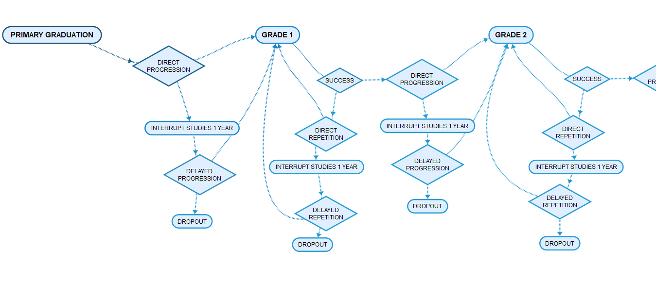
2.3.9.2. Parameters¶

Secondary Success: by grade. Proportion of students passing a grade.
Secondary Direct Progression Intake by grade. Proportion of students directly progressing to this grade after having passed the previous grade (or primary school in the case of grade one).
Secondary Delayed Progression Intake by grade. Proportion of students progressing to this grade after having interrupted studies for a year after passing the previous grade.
Secondary Direct Repetition Intake by grade. Proportion of students immediately repeating a grade after failing to pass.
Secondary Delayed Repetition Intake by grade. Proportion of students repeating a grade after having interrupted studies for a year after failing the previous grade.
Maximum years of delays allowed (interruption, repetition of grades): Sets the maximum time of delays in secondary studies. Any further delay leads to a permanent dropout.

2.3.9.3. Output Tables¶

Secondary school enrolment by grade
Secondary school attainments of population 20-24 by year and sex. Proportion of the population age 20-24 having entered / having completed secondary education

2.3.9.4. Scenario Examples¶

Improvements in secondary education entry and success: Estimates of secondary school entry rates, as well as repetition and success rates are available for most countries (e.g. from UNESCO at http://data.uis.unesco.org/) and can be used as base for scenarios of future improvements in secondary education.

2.3.10. Human Capital Index (and its components)¶

2.3.10.1. Model Overview¶

DYNAMIS-POP models all components of the World Bank’s Human Capital Index (HCI) and allows its calculation and projection on a disaggregated level, e.g. by region. The Human Capital Index measures the human capital that a child born today can expect to attain by age 18, given the risks to poor health and poor education that prevail in the country where she lives. The HCI follows the trajectory from birth to adulthood of a child born today.

Components of the HCI are:

Child survival up to the 5th birthday
Adult survival from 18 to 60
Years of schooling age 4-18 (max 14 years) including up to two years of pre-school
Quality of education to quality-adjust the years of schooling. This measure is based on test scores
Stunting in the first 5 years of life

While most of the components for calculating and projecting the HCI are already available from other modules of DYNAMIS-POP (mortality, primary education and secondary education; and detailed population projections in general), two components have to be added: stunting and preschool education.

The pre-school module is a simple module implementing up to 2 years of pre-school experience. It is assumed, that all children attending pre-school enter primary education. Pre-school experience is decided at school entry thus the career itself is not modeled. The module has one single parameter table containing the probability to have attended pre-school for at least one year, and the probability that the pre-school experience was two years (by sex and region).

Stunting is the impaired growth and development that children experience from poor nutrition, repeated infection, and inadequate psychosocial stimulation. Children are defined as stunted if their height-for-age is more than two standard deviations below the WHO Child Growth Standards median. Stunting is modeled as an individual level ‘fate’ decided at birth based on sex, region, and mother’s education.

On the population level, the HCI is calculated by multiplying up its components in the following form.

HCI = [Child Survival to 5th birthday]
      * exp(0.08 * ([average years of schooling] * [average quality of schooling] - 14))
      * exp((0.65 * ([adult_survival] - 1.0) + 0.35 * ([proportion children not stunted] - 1.0)) / 2.0);

The individual human capital can be calculated from the individual life experience - like the years of schooling - of each actor at the moment of her death. Note that, if the components of the human capital are correlated (which is the case as e.g. stunting affects school success) the average of the individual human capital will be different from the aggregate HCI calculated from the average values of the components.

2.3.10.2. Parameters¶

Stunting by mothers education, region and sex: This parameter is estimated from the analysis data.
Preschool attendance: by sex and region. This is a scenario parameter giving the probability of already having attended one or two years of preschool when entering primary school.
Quality of schooling by region. A scenario parameter used for weighting the years of school attendance.
HCI Coefficients: The coefficients used in the formula of the HCI

2.3.10.3. Tables¶

HCI variables by region of birth, sex and year of birth. A set of HCI related indicators: Stunting rate, Child survival rate, Adult survival rate, Average quality of schooling, Average years of schooling, Average individual level HCI.
HCI variables by district of birth, sex and year of birth. A set of HCI related indicators: Stunting rate, Child survival rate, Adult survival rate, Average quality of schooling, Average years of schooling, Average individual level HCI.
Stunting rates by region of birth, sex, and year of birth.

2.3.10.4. Scenario Examples¶

What-If Scenarios and Vulnerable Populations: DYNAMIS-POP allows to create what-if projections of the HCI and its components. Of particular interest (as benchmark for an assessment of policy effects) are status quo scenarios on the micro level. In such scenarios, all trends at the macro level result from a changing population composition, while for people belonging to a specific group (e.g by region, education, ethnicity) the factors entering HCI (mortality, stunting, education) remain unchanged. Other ‘popular’ what-if scenarios would address the differences between population groups and policies targeting specific vulnerable groups. For example, we might assess the impact of narrowing the education gap between population groups on the HCI.
Decomposition Analysis and Time-Lines of Policy Effects: DYNAMIS-POP allows a decomposition analysis of projected changes in the HCI. This analysis goes beyond the contribution of the individual components of the HCI, as we can assess which part of the changes within each component stem from composition effects.
Quantify the downstream effects of policies: For example, improvements in education influence the HCI not only directly (e.g. more years in school) but also impact child mortality and stunting. Microsimulation can measure these effects and project the timeline of improvements.
Sub-National Analysis: DYNAMIS-POP operates at the sub-national level allowing to assess local variations in the HCI and its components. Closing sub-national gaps is a typical policy goal and DYNAMIS-POP allows the geographical mapping of the HCI and other measures.
Projections of the Human Capital of the Actual Population: DYNAMIS-POP allows projections of the human capital of the actual population: the HCI is a cohort measure and does not allow to directly infer the future average human capital of the working age population. For example, high child mortality substantially lowers the HCI of a cohort but does not impact the human capital of the survivors who make the future work force. Also, as a macro index, the HCI is constructed by a formula linking together the population averages of the components of the measure. As the components are highly correlated at the micro level (e.g. stunting increasing child mortality, lowering education prospects, etc.) the HCI is not identical with the average human capital of the population. DYNAMIS-POP allows comparing the HCI with the average human capital of the simulated cohort. Being able to make statements on the average individual level human capital and its distribution might be valuable in economic modeling. In general, one of the strengths of DYNAMIS-POP is its ability to simultaneously produce various alternative measures and their distribution, which can then be picked according to the concrete research question.

2.3.11. Microdata Output¶

2.3.11.1. Overview¶

DYNAMIS-POP produces two types of micro-data (CSV) output. The first is a file of a pre-set collection of variables either produced once as a single cross-sectional file or repetitively as panel data. The time of the (first) output and the time intervals between outputs are specified by the user. The second microdata output produces four microdata files at a selected point in time. These four data files have the same format and content required to create a model starting population and to estimate all parameters using the set of analysis files documented and available at the Project Website. This file output is mainly used for model validation as it allows re-estimating all parameters based on simulated data. Both types of file output are optional and can be switched off.

2.3.11.2. Cross-sectional and Panel Micro-Data Output Parameters¶

Write micro-data output file Y/N
File name micro-data output file
Time(s) of micro-data output: The first point in time, the time intervals, the last point in time. If setting time intervals to 0 output is produced only once.

2.3.11.3. Analysis Data Output Parameters¶

Analysis file output Y/N
File name: Births:
File name: Children
File name: Emigrants
File name: Residents
Time of analysis file output: A single point in time. Note that the Birth file and the Children file contain retrospective histories which have to be created within the simulation. For complete birth records, the model has to be run over at least 40 years.

2.3.11.4. Output Files¶

Micro-Data: This file currently only contains a few variables and is used for demonstrational purposes only. The list of variables can be easily extended in the implementation code. Variables in DYNAMIS-POP 2.22 are: Record ID, Weight (identic for all), Time of output, Time of birth, Sex, District of residence, Education level.
Residents: A synthetic future census of the resident population. Variables are: Record ID, Household ID, Weight (identic for all), Age, Sex, District of birth, District of residence, District 12 months ago, Education, Parity, Births past 12 months, Age at marriage, Age at most recent birth, Region of birth, Region of residence, Region 12 months ago, Ethnicity.
Emigrants: Emigrants of the past 12 months. Variables: Weight (identic for all), district of residence (abroad for all), previous district, Previous region, Age, Sex.
Births: Retrospective birth histories for the analysis of fertility. Variables: Month birth 01 .. 14, Weight, Month of own birth, Education, Region, Month of interview, Month of first marriage, District
Children: Retrospective child records of births in the past 5 years for the analysis of child mortality, stunting, and child vaccination. Variables: Weight (identic for all), Month of interview, Region, Month of birth, Month of death, Sex, Age of mother (months) at birth, Education of mother, Ethnicity, Immunization, District, Prenatal care, Stunting.