1.7. Modules

This section describes the key processes and components of DYNAMIS-POP. The model is organized into modules which typically address a specific behavior or process (like mortality), correspond to a code file as well as an R script for parameter generation. The modules described in this section cover the key model components for producing simulations and can be classified into three groups.

• Core demographic modules: These are the modules necessary for the micro-simulation implementation of a typical cohort component population projection model. Without any other modules added, these core modules constitute a fully functional equivalent to common macro models, projecting populations by age, sex, and district. When combined with additional modules, the core modules can be used to produce alignment targets. This allows to produce the same aggregate population projections as in existing projections while creating realistic individual careers and adding detail like education, school attendance, ethnicity, and partnership status. Core demographic modules use the same parameters as macro models, like age-specific fertility, life tables, and transition matrices. Life tables and projected fertility rates are widely available for most countries for download. All migration parameters can also be produced from the micro-data files using the R scripts documented in this report (the scripts, or an updated version of them, are published in our Github repository)..
• Other core modules: These are the base versions of modules necessary for adding additional variables and related processes to the model. Examples are education, the intergenerational transmission of ethnicity, and first union formation. All parameters are produced based on the four required micro-data files running the R scrips documented in this report.
• Refined and optional modules: These are optional modules which refine existing modules or add functionality. These modules can be removed or replaced by customized modules. For example, the refined fertility modules uses information on partnership status, education and the timing and number of previous births. Refined models for child mortality and education account for mothers’ characteristics. Additional optional education modules track students through a grade system, add a secondary school system, and introduce functionality for school infrastructure planning. Most parameters are based on the four required micro-data files. Some parameters are scenario based. Both the data-based parameters as well as default scenario parameters are produced by the set of R scrips documented in this report.

1.7.1. Core Demographic Modules

1.7.1.1. The Starting Population

The model starts from a starting population file—a standard comma-separated variables (CSV) text file containing ten variables. Records can be weighted and the file length does not have to correspond to the true population size nor the size of the simulated population sample, which are parameters. According to these parameters, when the file is larger than the simulated starting sample, the model automatically samples from the starting population file. If the file is smaller than the chosen starting sample, the model replicates observations. All model output is automatically scaled to the total population size regardless of the chosen sample size for the simulation. Choosing larger samples will reduce Monte Carlo variability at the expense of additional time requirements to run the model.

The starting population and all parameters of the module are generated running the R “Script 2 - Starting Population”. Parameters are:

• The file name
• The file size
• The simulated sample size (which can be bigger or smaller than the file)
• The real population size (to which all output is automatically scaled)

The starting population has the following variables:

WEIGHT      Sample weight (123.456)
BIRTH       Year of birth (1956.789)
SEX         Sex (0 female, 1 male)
DISTRICT    District number 0..n
EDUC        Primary education ( 0 non, 1 incomplete, 2 completed)
DOB         District of birth (0..m, m = abroad)
UNION       Year of first marriage (1978.901)
PARITY      Number of births (0..)
LASTBIR     Year of last birth (1989.012)
ETHNO       Ethnicity (0..x)

1.7.1.2. The Core Mortality Module

Mortality is modeled by age and sex. Parameters are a mortality table (for age patterns) and projected period life expectancy. Within the application, the life table is scaled automatically for each year to meet the targeted life expectancy by calendar year and sex. The separation of parameters in age pattern and aggregated outcome in life expectancy supports easy scenario building and - in the case no national mortality projections are available - the use of regional standard mortality tables.

Parameters:

• Life table of mortality risks by age and sex
• Life expectancy for projected years by sex

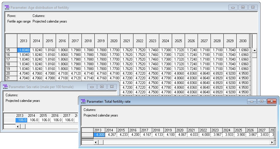
Figure: Mortality Parameters

Projections of life expectancy can have various sources: national projections, national goals, UN and U.S. census bureau projections, recent trends and international experience projections, or an application of the UN model schedule of mortality improvements. Data sets for individual countries and regions can be downloaded from various sources, including the DemProj project site. In the case of Demproj, two sets of model life tables are employed: the CoaleDemeny (Coale, Demeny, and Vaughan, 1983) model and the United Nations tables for developing countries (United Nations, 1982).

1.7.1.3. The Core Fertility Module

The fertility module is based on age-specific fertility rates calculated from two parameters: an age distribution of fertility and the TFR for future years. In this parameterization, the model directly follows the DemProj approach, which splits fertility projections into one of age patterns and another of TFRs. The third parameter is the sex ratio.

Modeling fertility exclusively by age does not result in a realistic representation of female birth histories or the observed distribution of family sizes as it ignores important other individual characteristics, like marital status, the current family size, education, and the time since last birth. Because of this limitation, even with perfect foresight, the model would only produce the right number of children but no realistic female life-courses.

The parameters of the module are:

• Age distribution of births by calendar year
• Total fertility rate by calendar year
• Sex ratio by calendar year

Figure: Fertility Parameters

The parameterization allows to easily change the scenario of the projected total fertility rates (TFR) without having to change the age profile of fertility. Internally, the model automatically calculates fertility rates by age and period.

The base fertility module is used in two alternative ways: as the model to be used to implement fertility, and as the benchmark model. In the latter case, it is used to produce the number of births to which the more detailed refined fertility model can be aligned.

Projections of fertility are provided online by multiple sources like national projections or UN and U.S. census bureau projections. Data sets for individual countries and regions can also be downloaded from the DemProj project site.

1.7.1.4. Internal Migration

Interprovincial migration is modeled by age group and sex. For easier scenario creation, probabilities to leave a district and distribution of destination districts by age group and origin are parameterized separately. It is assumed that migration pattern stay constant over time.

Parameters

• An on/off switch to activate/deactivate the module
• Probabilities to leave a district by age group and sex
• The distribution of destination districts by district of origin, age group, and sex

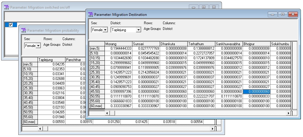
Figure: Internal Migration Parameters

The parameters are calculated from the micro-data files running the R “Script 5 - Internal Migration” provided with this report.

1.7.1.5. Emigration

The emigration module implements a typical macro approach driven by age-specific emigration rates by district and sex. It is assumed that emigration pattern stay constant over time.

Parameters:

• Switch emigration on/off
• Emigration rates by age, sex, and district

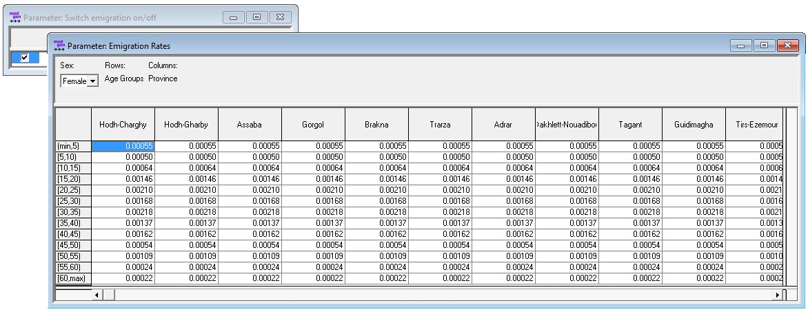
Figure: Emigration Parameters

The parameters are calculated from the micro-data files running the R “Script 6 - Emigration” provided with this report.

1.7.1.6. Immigration

The immigration module implements a typical macro approach, specifying the number of future immigrants, their age distribution, and the distribution of the district. Like residence, immigrants are modeled from birth and live abroad until entering the country. This approach gives maximum flexibility in modeling their characteristics. For example, in DYNAMIS-POP education attainments and progressions of immigrants are modeled like for nationals (“abroad” being treated like an additional district in parameters), whereas (in the refined fertility module) parity and time of last birth are sampled from the host population and imputed at the moment of arrival.

Parameters:

• Switch immigration on/off
• Total number of immigrants by sex and calendar year
• Age distribution of immigrants by single year of age, separately by sex
• Distribution of destination districts by sex and age group

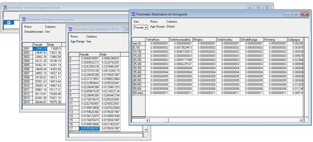
Figure: Immigration Parameters

The parameters are calculated from the micro-data files running the R “Script 7 - Immigration” provided with this report.

1.7.2. Other Core Modules

1.7.2.1. Base Primary Education Fate

Based on the information in the starting population and parameters by district, year of birth and sex, the final primary education outcome is decided at birth. The outcome has 3 possible levels:

• Never entered primary school
• Primary school dropout
• Primary school graduate

Probabilities to progress from low to medium and from medium to high are given by two parameters by year of birth, district of birth, and sex. The way the education fate is decided depends on the year of birth and the person type. For persons from the starting population the education outcome is taken from the starting population file for people who - given their age - it can be assumed that the primary education career is finished, otherwise the final outcome is modeled. For immigrants based on their year of birth the education fate is either modeled or sampled from foreign born residents born in the previous 12 months.

Parameters:

• Probability to enter primary school by year and district of birth and sex
• Probability to graduate from primary school by year and district of birth and sex

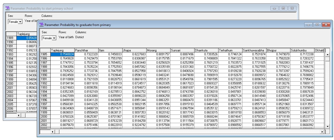
Figure: Primary Education (base) Fate Parameters

All parameters are estimated from the micro-data files using logistic regression running the R “Script 8 - Primary Education Fate” documented in this report. The model includes a trend variable (logarithmic, thus levelling off with time) which is used in the default scenario for which parameter tables are created by the script. While estimated as log odds, parameters are expressed as probabilities allowing for easy scenario creation.

1.7.2.2. Ethnicity

The concept of ethnicity is generic / country specific. Ethnicity can refer to any grouping of the population and could represent ethnical background, caste, or religion. Parameters are the transmission of the ethnicity variable from mother to child and the ethnicity distribution of immigrants by age and sex.

Parameters:

• Ethnic transmission from mother to child by sex of child and mothers ethnicity
• Ethnicity distribution of immigrants by sex and destination district

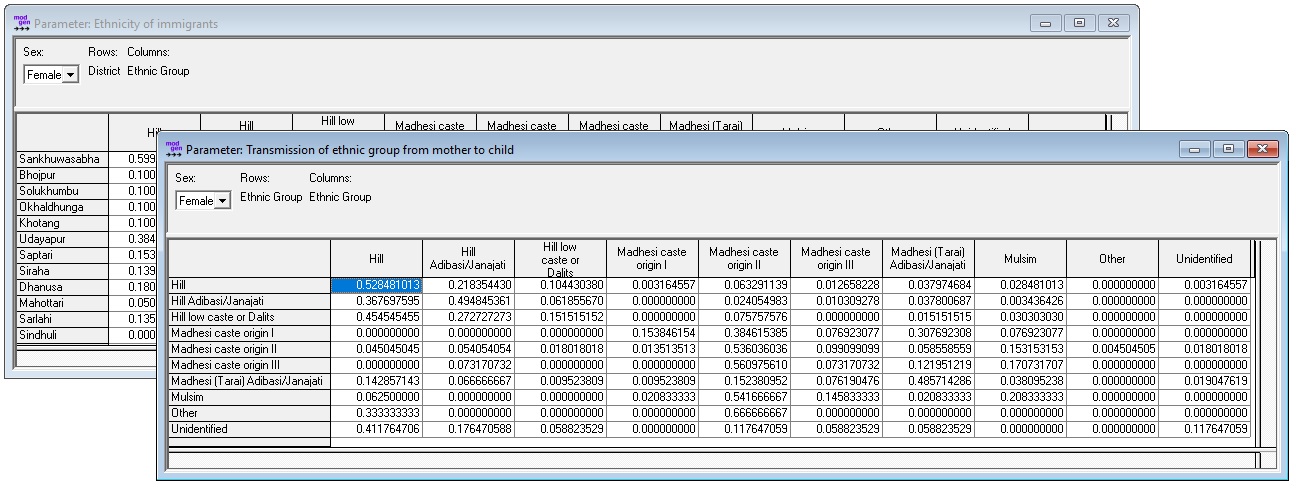
Figure: Ethnicity Parameters

The parameters are calculated from the micro-data files running the R “Script 10 - Ethnicity” provided with this report.

1.7.2.3. First Marriage

Changes in the age at first union formation is one of the key mechanisms behind fertility changes. Many developing societies currently experience a rapid increase in that age, partly resulting from educational expansion. Including this variable in the fertility model allows a better depiction of the concentration of reproduction: instead of distributing children to women independent of union status, fertility will be more concentrated to fewer women, especially at young ages, which better reflects reality.

From a modeling perspective, the fast-changing age profile in first union formation poses interesting challenges. Fast demographic change, especially shifts in age profiles, make period data of limited use for modeling. For example, union formation rates decrease fast for the very young, but this observation does not necessarily mean that fewer people enter a union over the life-course, even if union formation rates are currently low at higher ages, where most of people observed today have entered a union already. It is in such environment that parametric models demonstrate their power. We implemented the Coale & McNeil approach for modeling entry into first unions. The parameterization of such a model is very intuitive; parameters are the minimum age at first union formation, the average age, and the proportion of women who will eventually marry. The model was proposed by Coale and McNeil in the 1970s, based on extensive studies on the age pattern of first marriages in many countries. Their standard density of first marriage, constructed from pattern observed in Sweden 1856-9, has the form:

gs(x) = 0.19465*exp(-0.174(x-6.06) – exp(-0.288(x – 6.06)))

They found that a relational model with three parameters transforming the proportion of ever married at the age resulting from the above density function can fit most populations:

G(a) = C * GS ( ( a-a0 ) / k )

• a = age
• a0 = minimum age when the process starts (empirically, ~age where the first percent married)
• k = indicator of the spread of the distribution, i.e., how fast marriage occurs after a0 (how many years of the population’s schedule are equivalent to one year of the standard)
• C = the proportion of the population eventually entering marriage

Rodriguez and Trussell (1980) noted that k stands in direct relation to the average age at marriage µ, allowing parameterizing a model more intuitively with µ instead of k:

µ = ∫aG(a)da = a0+11.36k, thus k = (µ - a0)/11.36

Parameters:

• Earliest age of marriage, average age at first marriage, and proportion of women eventually married by year of birth and primary education attainment. (Coale & McNeil Model)

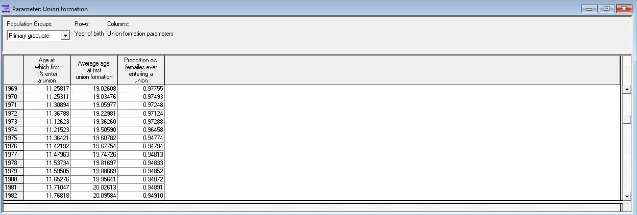
Figure: First Marriage Parameters

All parameters are estimated from the micro-data fitting Coale & McNeil models by the R “Script 11 - First Marriage” provided with this report. For the future linear trends are created informed by the past and used in the default scenario for which parameter tables are created by the script. These trends can easily be modified by users for creating alternative scenarios.

1.7.3. Refined and Optional Modules

1.7.3.1. Refined Primary Education Fate

This module introduces the option of modeling inter-generational transmission of education. It adjusts the overall probabilities from the base module to enter and graduate from school by a set of relative factors (odds ratios) by mother’s education. Users are given a choice if and how the refined model is used. One option consists in calibrating the aggregate outcomes by sex and district to the base model for all years of birth. In this case, aggregate outcomes remain the same, but the more likely children are chosen to enter and graduate from school. This might be of value when studying the school (and out of school) population by socio-demographic characteristics. The second option calibrates the model just for one birth cohort from which onward the refined module is used. All simulated future trends are then driven entirely by composition effects. These model capabilities allow educational change to be decomposed into changes stemming from inter-generational dynamics, from inter-provincial migration, and from overall trends.

Parameters:

• Model selection: the 3 options are (1) base model, (2) refined model calibrated for all years of birth, (3) refined model calibrated once.
• Odds for starting primary education by mother’s education
• Odds for graduating from primary education by mother’s education
• The first birth cohort from which onwards the refined model is used, which can be any year beginning from the starting year of the simulation.

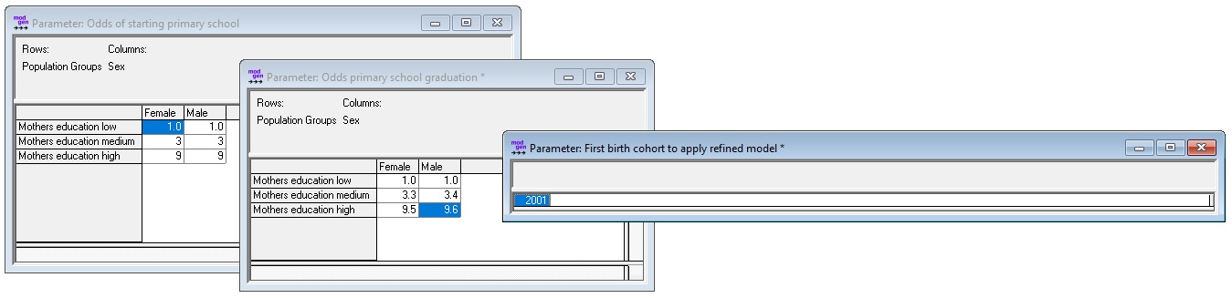
Figure: Primary Education Refined Fate Parameters

The module can be added or removed from the model without requiring modification in other modules. All parameters are estimated from the micro-data running the R “Script 09 - Primary Education Refined Fate”.

Variants: This module is currently implemented in two versions, the first corresponding to the module described above, the second additionally adding relative factors for the influence of stunting on school entry and outcome.

1.7.3.2. Refined Fertility

While very popular, the use of period rates of age-specific fertility in population projections has three types of limitations:

• Even if it were possible to have perfect knowledge of future rates, the simulation would not produce realistic life-courses for women. Age as the only determinant of fertility would not lead to a realistic distribution of children to mothers and thus of family sizes. It ignores other determinants of fertility like parity, time of the last birth, union status, and education. So even with perfect foresight, we would obtain only the right number of babies. Micro-simulation can increase policy relevance of projections by placing newborns into their family context: their survival, future school attendance, etc., can take into account parents’ characteristics, which in return are relevant to the cost of policies.
• A projection tool based on age-specific rates cannot inform scenarios of fertility changes. Scenarios must be produced outside of the model, and often mechanically, by starting from observed rates, future target rates (e.g., from a country which underwent demographic changes earlier), and a transition path. Theories of behavioral changes are not made explicit nor are they distinguishable from composition changes. Micro-simulation allows the explicit modeling of behavioral changes, respectively, permits the study of composition effects in isolation. The latter can run status quo scenarios where changes in overall fertility arise entirely from changing composition of the population.
• Macro scenarios based on given rates do not allow modeling of feedback reactions and policy effects on fertility. For example, if highly educated women are expected to have fewer and later births, a micro-simulation model will naturally produce these downstream effects when running scenarios on educational expansion. Other scenarios could include legislation effects, e.g., the imposition of a minimum age of marriage.

The refined fertility module was built to address these issues. First, we model births separately by birth order. In the case of first birth, age is kept as the main (baseline) factor, but age-specific birth rates are estimated separately by education group (expecting differences in the age pattern) and for women who ever entered a union and those did not (where fertility is very low).

For higher-order births, we estimate separate models for births of order 2-15. To model realistic birth intervals, the baseline is now the time since previous birth. Relative risks were added to capture the effects of education and broad age groups, as for higher ages fertility decreases considerably.

Users are given various model choices for model selection and alignment options. In particular, the refined model can be run with total births or total births by age aligned with the base model. This produces identical aggregate projections as found in published sources while respecting the relative differences in birth risks between women by parity, birth interval, education, and union status.

Simulated birth events only occur to residents in the projected time, as biographic information on parity and the most recent time of birth are contained in the starting population. As for immigrants no biographic information is available, immigrant women sample parity and timing of last birth from the female resident population of same education and partnership status and district.

Parameters:

• Model selection: 4 options, base model, refined model, refined model aligned to number of births of base model, refined model aligned to number of births by age of base model.
• First births rates by education, region, partnership status, age.
• Higher order births: hazard regression parameters with a duration baseline (age; time since last birth) and relative risks for education and age group.
• Birth trends: an additional relative risk by calendar year and parity.

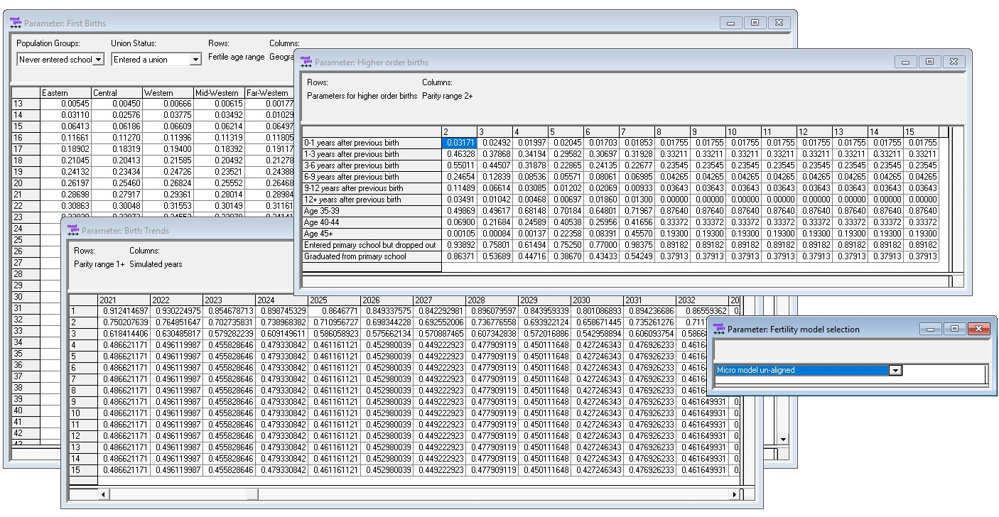
Figure: (Refined) Fertility Parameters

Estimation of first birth rates:

First births are based on the file of residents typically generated from census data using the information on reported births in the past 12 months. Parameters are birth rates (hazards) by single year of age and province of residence, marital status (ever having entered a union), and the three education groups based on primary school entry and graduation. While the parameter consists of a single four-dimensional table, i.e., age, province, marital status, education, the respective rates are calculated from the log odds estimated using logistic regression models:

• For women 15+ who ever entered a marriage, models by age and province are run separately for each education group, allowing for different age profiles by education.
• For women 15+ who never entered a marriage, due to a much smaller population and very low birth rates, education is added as proportional factor instead of estimating the model separately by education.
• Fertility below age 15 is estimated separately, as the influence of education and regional differences are different at this young age compared to women 15+.
• The models for first births of women below age 15 are estimated separately by marital status. Due to very small sample/population, inter-provincial differences are not estimated for women who never entered a marriage.

All first birth parameters are estimated and generated running the R “Script 12 - First Births” provided with this report.

Estimation of higher order births

For the second to the 14th birth, separate proportional (piecewise constant) hazard regression models are estimated from the file of birth records which is typically compiled from survey data like MICS or DHS. This approach was chosen as the duration since last birth is a strong predictor of higher-order birth events and including this duration, which is not available from the census, allows more realistic modeling of birth intervals and thus female life-courses.

All higher order birth parameters are estimated and generated running the R “Script 13 - Higher Order Births” provided with this report.

This module can be added or removed from the model without any code change to other modules.

1.7.3.3. Child Mortality

Child mortality is a key policy concern in many developing countries. There is a wide body of literature on determinants, both individually, e.g., characteristics of the mother, and contextually, e.g., availability of health care infrastructure on the regional level. Micro-simulation can be a powerful tool for policy-relevant analysis and projections, as it can handle the detailed characteristics that drive child mortality. In this context, the presented model is just a starting point for detailed analysis. It takes two characteristics of mothers into account, mother’s age and education.

This module implements infant and child mortality (at ages 0-4). The child mortality module is based on a proportional hazard regression model consisting of (1) a mortality baseline by age and sex, (2) relative risks by age for mother’s age group at birth and mother’s education, and (3) a time trend by age (which can be chosen to be applied overriding the general mortality trends of the base model)

The module is optional, and the user can choose between various options:

• Disable the child mortality model: the same model as for all ages is used.
• Child mortality model without alignment: the child mortality module replaces the overall mortality module for ages 0-4.
• Child mortality model calibrated for an initial year, then trends as for other ages: In this choice, life expectancy is the same as in the overall mortality for the given year, but as the composition of the population by mothers’ characteristics changes over time, the number of deaths (and therefore life expectancy) will be different for the following years, allowing for scenario comparisons.
• Child mortality model calibrated for an initial year, then specific trends from the child mortality module: In this choice, life expectancy is the same as in the overall mortality for the given year, but as the composition of the population by mothers’ characteristics changes over time, and as a result from potentially different trends, the number of deaths (and therefore life expectancy) will be different for the following years, allowing for scenario comparisons.

If activated, the model for child mortality starts replacing the overall mortality model five calendar years after the starting year of the simulation, which is when the first five cohorts of babies are born in the simulation and are then age 0-4. As mother’s characteristics are not available for children born outside the country, immigrants are excluded from the model and handled by the general mortality module.

Parameters:

• Model Selection
• Mortality baseline hazards by age and sex
• Mortality relative risks by age and mother’s characteristics (age and education)
• Time trend

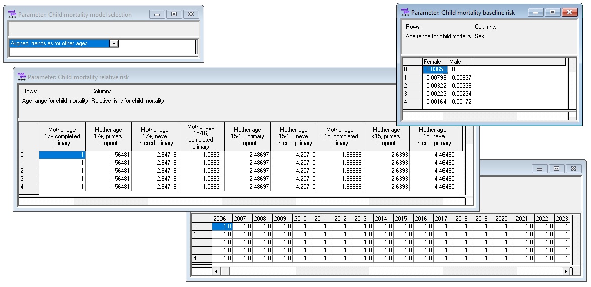
Figure: Child Mortality Parameters

All Parameters of this module are estimated and generated running the R “Script 14 - Child Mortality”.

1.7.3.4. Primary Education Tracking

This is an optional module used to track students through the primary education grade system. The number of grades is country specific and can be adapted to different school systems. At the end of each school season it is decided who newly enters the school at grade one, who of the active students passed the attended grade, who graduated, who permanently leaves school, and for all others if enrollment is continued or the school career is interrupted by one year. The module builds on the fate model of school entry and success, thus only models the careers of those fated to enter school. Those fated to graduate from school at some point pass all grades. Those fated to drop out accordingly do not pass all grades - the distribution of the highest grade attended being a model parameter.

The module is driven by 6 parameters:

• The distribution of school entry ages by year of birth. Even in presence of a legislated school entry age, data in some developing countries reflect a wider range of ages when school is first entered. This parameter allows to account for that fact and allows for scenarios in which school entry ages become more concentrated toward the legislated age.
• The start of the school year: e.g. 0.666 for September 1st
• The end of the school year: e.g. 0.5 for June 30
• A grade repetition rate. The probability that a grade has to be repeated.
• A school interruption rate. The probability that the school career is interrupted for a year.
• The distribution of the highest grade attended of dropout students.

Besides grade and period, the school progression parameters have two additional dimensions, one for geographical region, the other for personal characteristics. The levels of these two characteristics are model specific. Currently only totals are implemented.

Figure: Primary Education Grade Tracking Parameters

As an optional module the module can be added or removed from the model. Different to most other modules, the parameters of this module are not estimated or calculated from the micro-data sets but scenarios have to be created by the user, e.g. using progression rates as published by UNESCO. Default parameter tables are generated running the R “Script 15: Primary Education Tracking” provided with this report.

1.7.3.5. School Planning

This module is an add-on to the primary education module used for planning of necessary school infrastructure investments. Based on parameters of current and future target teacher to student ratios and classroom sizes, it calculates the number of teachers and classrooms required for each calendar year and district.

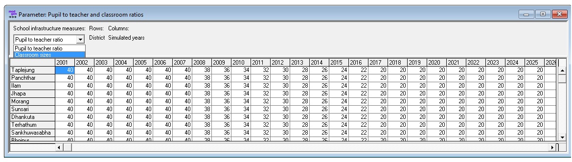
Figure: Primary Education School Planning Parameters

The module is optional and can be remove without damage to the model. Different to most other modules, the parameters of this module are not estimated or calculated from the micro-data sets but scenarios have to be created by the user. Default parameter tables are generated running the R “Script 16: School Planning” provided with this report.

1.7.3.6. Lower Secondary Education

This is an optional module for modeling a secondary school which can be attended after graduating from primary education. The number of grades is country-specific. The model follows a period approach. Each year at the end and beginning of school season it is decided if a person enters school, succeeds a grade, progresses to the next or repeats a grade, interrupts studies or permanently drops out. A parameter controls the maximum number of years which can be delayed due to repetition or temporary dropout. A student interrupting education can resume studies after a year or stay out permanently. The model is driven by parameters for each calendar year and grade:

• The probability to pass a grade
• The probability to move on directly after passing a grade
• The probability to repeat a grade immediately after failing it
• The probability to resume studies after being out for a year after passing a grade
• The probability to repeat a grade after being out for a year after failing a grade
• The maximum number of years studies can be delayed by repetition or inactive spells

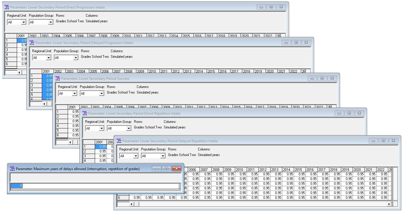
Figure: Secondary Education Parameters

Besides grade and period, the school progression parameters have two additional dimensions, one for geographical region, the other for personal characteristics. The levels of these two characteristics are country specific. Currently only totals are implemented.

As an optional module the module can be added or removed from the model. Different to most other modules, the parameters of this module are not estimated or calculated from the micro-data sets but scenarios have to be created by the user, e.g. using progression rates as published by UNESCO. Default parameter tables are generated running the R “Script 17: Lower Secondary” provided with this report.

1.7.3.7. Pre-School Education

The pre-school module is a simple module implementing up to 2 years of pre-school experience. This module is an add-on developed when introducing the calculations of the Human Capital Index (HCI). It is assumed, that all children attending pre-school enter primary education. Pre-school experience is decided at school entry thus the career itself is not modeled. The module has one single parameter table containing - by sex and region - the probability to have attended pre-school for at least one year, and the probability that the pre-school experience was two years.

1.7.3.8. Stunting

Stunting is the impaired growth and development that children experience from poor nutrition, repeated infection, and inadequate psychosocial stimulation. Children are defined as stunted if their height-for-age is more than two standard deviations below the WHO Child Growth Standards median. This module implements stunting as an individual level ‘fate’ decided at birth based on sex, region, and mother’s education.

1.7.3.9. Human Capital and the Human Capital Index HCI

This module calculates the components of the Human Capital Index and individual human capital. The Human Capital Index (HCI) measures the human capital that a child born today can expect to attain by age 18, given the risks to poor health and poor education that prevail in the country where she lives. The HCI follows the trajectory from birth to adulthood of a child born today.

Components:

• Child survival up to the 5th birthday
• Years of schooling age 4-18 (max 14 years) including up to two years of pre-school
• Quality of education to quality-adjust the years of schooling. This measure is based on test scores
• Stunting in the first 5 years of life
• Adult survival from 18 to 60.

Formula:

On the population level, the HCI is calculated by multiplying up its components in the following form.

HCI  = [Child Survival to 5th birthday]
         * exp(0.08 * ([average years of schooling] * [average quality of schooling] - 14))
         * exp((0.65 * ([adult_survival] - 1.0) + 0.35 * ([proportion children not stunted] - 1.0)) / 2.0);

The individual human capital can be calculated from the individual life experience of each actor at the moment of her death. Note that, if the components of the human capital are correlated (which is the case as e.g. stunting affects school success) the average of the individual human capital will be different from the aggregate HCI calculated from the average values of the components. At the individual level, the individual human capital IHC is:

IHC  = [survived first five years of life y/n]
         * exp(0.08 * ([individual years of schooling] * [individual quality of schooling] - 14))
         * exp((0.65 * ([proportion of time age 18-60 survived] - 1.0) + 0.35 * ([not stunted age 0-4 y/n] - 1.0)) / 2.0);

The Human Capital Index module implements the calculation of some of the components of the index as well as the index itself. Most components are addressed in dedicated separate modules or can be derived from recorded life course information stemming from other modules, e.g. schooling and survival.

1.7.3.10. Child Vaccination (Immunization)

This module implements child vaccination. A child is assumed to be immunized if it received a set of vaccines during the first year of life. Immunization is decided at birth and depends on a set of individual and mother’s characteristics. The set of characteristics is country-specific and typically includes sex, mother’s education, region, and ethnicity. An important predictor for child vaccination is whether the mother has received prenatal care. Therefore, in a first step, prenatal care receipt is decided.

The model has two parameters - Prenatal Care Odds and Child Vaccination Odds - which contain a set of odds of receiving prenatal care respectively all required vaccines. These odds are typically estimated by logistic regression. Immunization is decided according these models for all children born as residents during the simulation. Children born abroad during the simulation sample the immunization status of resident 0 year old peers living in the region assigned to them as region of entry.