4.2. Script 2: Age Pyramids by Education
This script produces age pyramids by education for the first and last year contained in the data. Pyramids are generated by district as well as on the national level. The output is based on two data files, one for a base, the second for an alternative scenario.
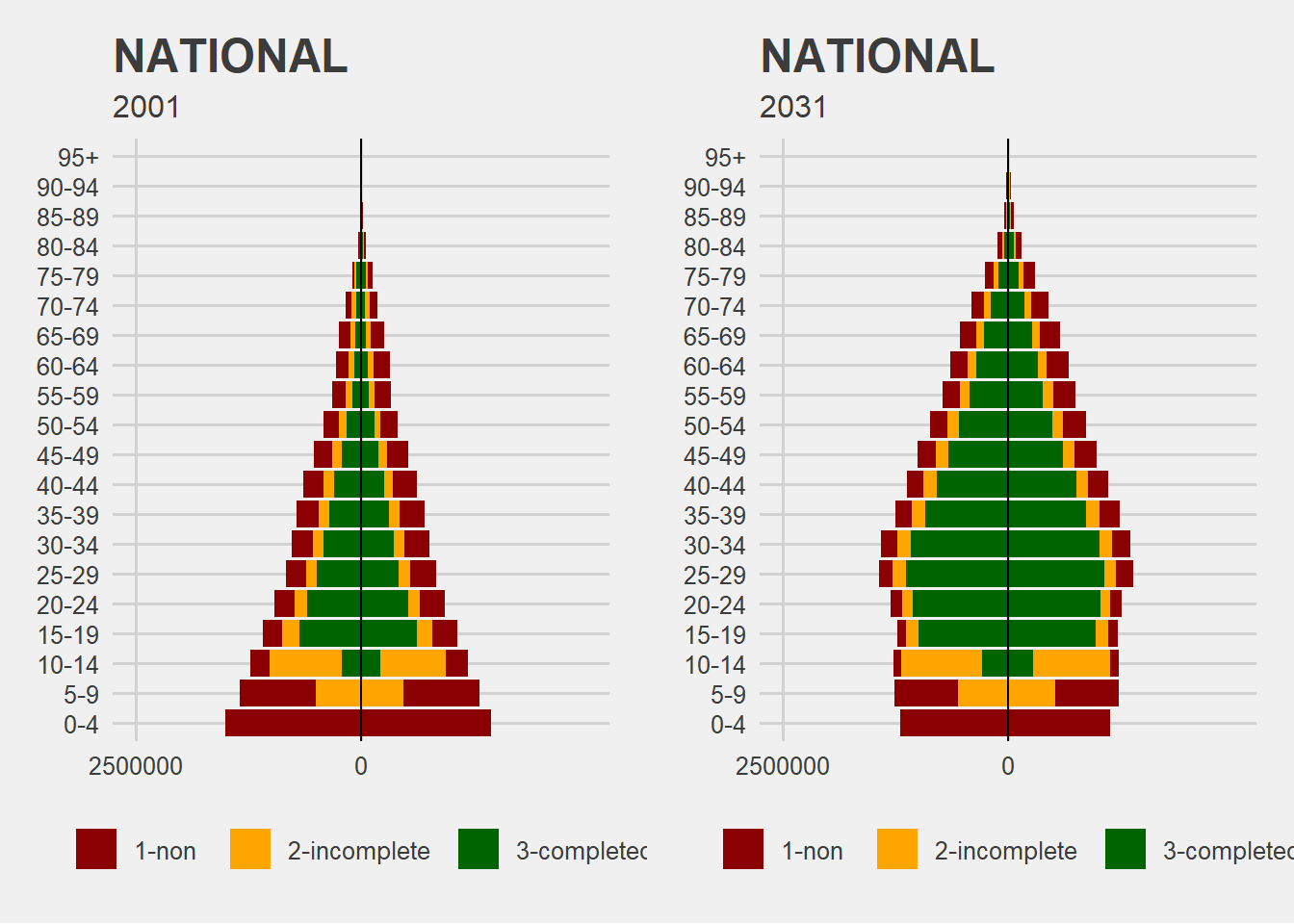
4.2.1. Base Scenario At Two Points in Time
####################################################################################################
#
#  DYNAMIS-POP Output Analysis File 2 - Chunk 1 - Population Pyramids by Education Base Scenario
#  This file is generic and works for all country contexts.
#  Input file: globals_for_output_analysis.RData (To generate such a file run the setup script)
#  Last Update: Martin Spielauer 2019-04-04
#
####################################################################################################

####################################################################################################
# Clear work space, load required packages and the input object file
####################################################################################################

rm(list=ls())

library("dplyr")
library("tidyr")
library("ggplot2")
library("ggthemes")
library("cowplot")

load(file="globals_for_output_analysis.RData")
time_one <- min(as.numeric(levels(unique(g_pyramid$g_data.TIME))))
time_two <- max(as.numeric(levels(unique(g_pyramid$g_data.TIME))))

####################################################################################################
# Create Population Pyramids - National
####################################################################################################

g1 <- ggplot(data = g_pyramid, aes(x = age, y = Freq, fill = educ)) +
geom_bar(data = g_pyramid %>% filter(gender == "female" & g_data.TIME == time_one
                                     & g_data.g_scenario == "base") %>%
       arrange(rev(educ)),
       stat = "identity",
       position = "stack") +
geom_bar(data = g_pyramid %>% filter(gender == "male" & g_data.TIME == time_one
                                     & g_data.g_scenario == "base") %>%
       arrange(rev(educ)),
       stat = "identity",
       position = "stack",
       mapping = aes(y = -Freq)) +
coord_flip() +
scale_y_continuous(labels = abs, limits = c(-12500000, 12500000), breaks = seq(-12500000, 500000, 12500000)) +
#scale_y_continuous(labels = abs) +
geom_hline(yintercept = 0) +
theme_fivethirtyeight() +
scale_fill_manual(values = c("darkred", "orange", "darkgreen")) +
labs(fill = "", x = "", y = "")
g1 <- g1 +  ggtitle("NATIONAL", time_one)

g2 <- ggplot(data = g_pyramid, aes(x = age, y = Freq, fill = educ)) +
geom_bar(data = g_pyramid %>% filter(gender == "female" & g_data.TIME == time_two
                                     & g_data.g_scenario == "base") %>%
       arrange(rev(educ)),
       stat = "identity",
       position = "stack") +
geom_bar(data = g_pyramid %>% filter(gender == "male" & g_data.TIME == time_two
                                     & g_data.g_scenario == "base") %>%
       arrange(rev(educ)),
       stat = "identity",
       position = "stack",
       mapping = aes(y = -Freq)) +
coord_flip() +
scale_y_continuous(labels = abs, limits = c(-12500000, 12500000), breaks = seq(-12500000, 500000, 12500000)) +

#scale_y_continuous(labels = abs) +
geom_hline(yintercept = 0) +
theme_fivethirtyeight() +
scale_fill_manual(values = c("darkred", "orange", "darkgreen")) +
labs(fill = "", x = "", y = "")
g2 <- g2 +  ggtitle("NATIONAL", time_two)

print(plot_grid(g1, g2, ncol = 2, nrow = 1))

####################################################################################################
# Create Population Pyramids - By District
####################################################################################################

for (nDistrict in unique(g_pyramid$sDistrict))
{
    g1 <- ggplot(data = g_pyramid, aes(x = age, y = Freq, fill = educ)) +
    geom_bar(data = g_pyramid %>% filter(gender == "female" & g_data.TIME == time_one
                                   & sDistrict == nDistrict & g_data.g_scenario == "base")
           %>% arrange(rev(educ)),
           stat = "identity",
           position = "stack") +
    geom_bar(data = g_pyramid %>% filter(gender == "male" & g_data.TIME == time_one
                                   & sDistrict == nDistrict & g_data.g_scenario == "base")
           %>% arrange(rev(educ)),
           stat = "identity",
           position = "stack",
           mapping = aes(y = -Freq)) +
    coord_flip() +
    scale_y_continuous(labels = abs, limits = c(-1500000, 1500000), breaks = seq(-1500000, 500000, 1500000)) +
    #scale_y_continuous(labels = abs) +
    geom_hline(yintercept = 0) +
    theme_fivethirtyeight() +
    scale_fill_manual(values = c("darkred", "orange", "darkgreen")) +
    labs(fill = "", x = "", y = "")
    g1 <- g1 +  ggtitle(nDistrict, time_one)

    g2 <- ggplot(data = g_pyramid, aes(x = age, y = Freq, fill = educ)) +
    geom_bar(data = g_pyramid %>% filter(gender == "female" & g_data.TIME == time_two
                                   & sDistrict == nDistrict & g_data.g_scenario == "base")
           %>% arrange(rev(educ)),
           stat = "identity",
           position = "stack") +
    geom_bar(data = g_pyramid %>% filter(gender == "male" & g_data.TIME == time_two
                                   & sDistrict == nDistrict & g_data.g_scenario == "base")
           %>% arrange(rev(educ)),
           stat = "identity",
           position = "stack",
           mapping = aes(y = -Freq)) +
    coord_flip() +
    scale_y_continuous(labels = abs, limits = c(-1500000, 1500000), breaks = seq(-1500000, 500000, 1500000)) +

    #scale_y_continuous(labels = abs) +
    geom_hline(yintercept = 0) +
    theme_fivethirtyeight() +
    scale_fill_manual(values = c("darkred", "orange", "darkgreen")) +
    labs(fill = "", x = "", y = "")
    g2 <- g2 +  ggtitle(nDistrict, time_two)

    print(plot_grid(g1, g2, ncol = 2, nrow = 1))
}
SAMPLE OUTPUT FROM THE IMAGINARY COUNTRY ABC
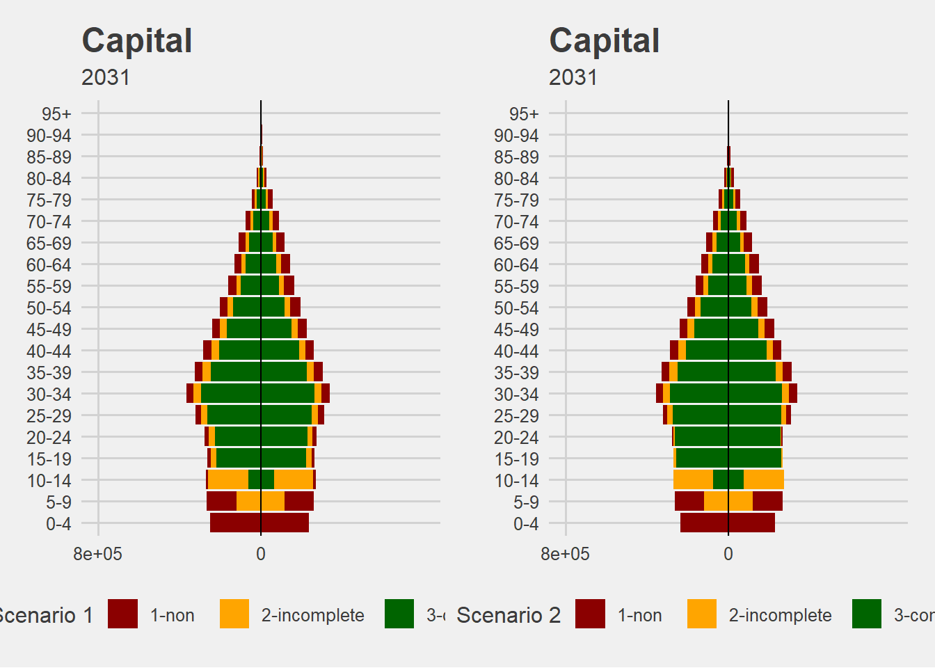
4.2.2. Age Pyramids by Education - 2 Scenarios
This script produces age pyramides by education comparing two educational scenarios. The graphs are produced for the last year in the projected data output file.
####################################################################################################
#
#  DYNAMIS-POP Output Analysis File 2 - Chunk 2 - Population Pyramids 2 Scenarios
#  This file is generic and works for all country contexts.
#  Input file: globals_for_output_analysis.RData (To generate such a file run the setup script)
#  Last Update: Martin Spielauer 2018-07-27
#
####################################################################################################

####################################################################################################
# Create Population Pyramids - National
####################################################################################################

g1 <- ggplot(data = g_pyramid, aes(x = age, y = Freq, fill = educ)) +
geom_bar(data = g_pyramid %>% filter(gender == "female" & g_data.TIME == time_two
                                     & g_data.g_scenario == "base") %>%
       arrange(rev(educ)),
       stat = "identity",
       position = "stack") +
geom_bar(data = g_pyramid %>% filter(gender == "male" & g_data.TIME == time_two
                                     & g_data.g_scenario == "base") %>%
       arrange(rev(educ)),
       stat = "identity",
       position = "stack",
       mapping = aes(y = -Freq)) +
coord_flip() +
scale_y_continuous(labels = abs, limits = c(-2500000, 2500000), breaks = seq(-2500000, 500000, 2500000)) +
#scale_y_continuous(labels = abs) +
geom_hline(yintercept = 0) +
theme_fivethirtyeight() +
scale_fill_manual(values = c("darkred", "orange", "darkgreen")) +
labs(fill = "Scenario 1", x = "", y = "")
g1 <- g1 +  ggtitle("NATIONAL", time_two)

g2 <- ggplot(data = g_pyramid, aes(x = age, y = Freq, fill = educ)) +
geom_bar(data = g_pyramid %>% filter(gender == "female" & g_data.TIME == time_two
                                     & g_data.g_scenario == "alt") %>%
       arrange(rev(educ)),
       stat = "identity",
       position = "stack") +
geom_bar(data = g_pyramid %>% filter(gender == "male" & g_data.TIME == time_two
                                     & g_data.g_scenario == "alt") %>%
       arrange(rev(educ)),
       stat = "identity",
       position = "stack",
       mapping = aes(y = -Freq)) +
coord_flip() +
scale_y_continuous(labels = abs, limits = c(-2500000, 2500000), breaks = seq(-2500000, 500000, 2500000)) +
#scale_y_continuous(labels = abs) +
geom_hline(yintercept = 0) +
theme_fivethirtyeight() +
scale_fill_manual(values = c("darkred", "orange", "darkgreen")) +
labs(fill = "Scenario 2", x = "", y = "")
g2 <- g2 +  ggtitle("NATIONAL", time_two)

print(plot_grid(g1, g2, ncol = 2, nrow = 1))

####################################################################################################
# Create Population Pyramids - By District
####################################################################################################

for (nDistrict in unique(g_pyramid$sDistrict))
{
    g1 <- ggplot(data = g_pyramid, aes(x = age, y = Freq, fill = educ)) +
    geom_bar(data = g_pyramid %>% filter(gender == "female" & g_data.TIME == time_two
                                   & sDistrict == nDistrict & g_data.g_scenario == "base")
           %>% arrange(rev(educ)),
           stat = "identity",
           position = "stack") +
    geom_bar(data = g_pyramid %>% filter(gender == "male" & g_data.TIME == time_two
                                   & sDistrict == nDistrict & g_data.g_scenario == "base")
           %>% arrange(rev(educ)),
           stat = "identity",
           position = "stack",
           mapping = aes(y = -Freq)) +
    coord_flip() +
scale_y_continuous(labels = abs, limits = c(-800000, 800000), breaks = seq(-800000, 500000, 800000)) +
# scale_y_continuous(labels = abs) +
    geom_hline(yintercept = 0) +
    theme_fivethirtyeight() +
    scale_fill_manual(values = c("darkred", "orange", "darkgreen")) +
    labs(fill = "Scenario 1", x = "", y = "")
    g1 <- g1 +  ggtitle(nDistrict, time_two)

    g2 <- ggplot(data = g_pyramid, aes(x = age, y = Freq, fill = educ)) +
    geom_bar(data = g_pyramid %>% filter(gender == "female" & g_data.TIME == time_two
                                   & sDistrict == nDistrict & g_data.g_scenario == "alt")
           %>% arrange(rev(educ)),
           stat = "identity",
           position = "stack") +
    geom_bar(data = g_pyramid %>% filter(gender == "male" & g_data.TIME == time_two
                                   & sDistrict == nDistrict & g_data.g_scenario == "alt")
           %>% arrange(rev(educ)),
           stat = "identity",
           position = "stack",
           mapping = aes(y = -Freq)) +
    coord_flip() +
scale_y_continuous(labels = abs, limits = c(-800000, 800000), breaks = seq(-800000, 500000, 800000)) +
#    scale_y_continuous(labels = abs) +
    geom_hline(yintercept = 0) +
    theme_fivethirtyeight() +
    scale_fill_manual(values = c("darkred", "orange", "darkgreen")) +
    labs(fill = "Scenario 2", x = "", y = "")
    g2 <- g2 +  ggtitle(nDistrict, time_two)

    print(plot_grid(g1, g2, ncol = 2, nrow = 1))
}
SAMPLE OUTPUT FROM THE IMAGINARY COUNTRY ABC